Solver
Solver infers one deterministic state-machine candidate from positive chronological observations. It keeps observation editing, inference, review, and replacement separate so no inferred model enters the project without explicit approval.
What the Solver Does
Solver normalizes typed observation tokens, builds an evidence graph, and applies deterministic constrained state merging. A successful result is one reproducible candidate consistent with every hard observation. Before offering it for review, Automata Lab validates the candidate and replays every sample against it.
Solver can use explicitly observed state identities and may invent stable generated states when the evidence requires hidden structure. Unobserved state-and-event combinations remain undefined rather than being filled with guessed transitions.
Solver Limitations
Finite positive observations generally do not identify one uniquely correct hidden machine. Solver therefore does not claim that its candidate is the real system or globally state-minimal.
The inference assumes that:
- all observations are hard constraints and contain no noise to repair;
- observed action blocks are complete and correctly ordered;
- observed event tokens form the complete event alphabet;
- observed action tokens form the complete action alphabet;
- different explicitly named states are different identities; and
- additional unnamed states may exist.
Generated candidates use entry actions only. Exit-action mappings are empty because the observation grammar describes the complete action word of the state reached after an event.
Observation Sequences
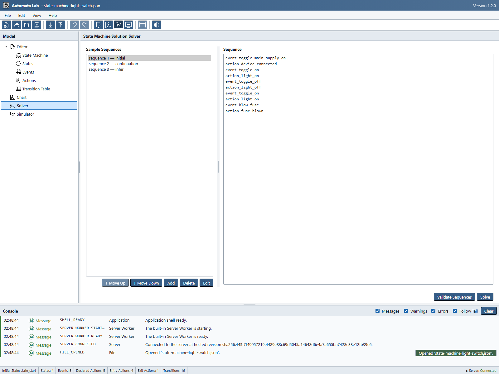
The left pane contains named Sample Sequences and the right pane contains a one-token-per-line Sequence editor. When the saved library is empty, an unsaved observation_1 sample with Infer context remains available. Solve uses every sample in the library, including the current editor text; selecting a row only chooses which sample to edit.
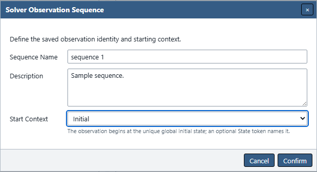
Use Move Up, Move Down, Add, Delete, and Edit beneath the sample list. Add and Edit manage a unique Name, optional Description, and Start Context. Sample order is cosmetic; token order within each sample is semantic.
Selecting a sample loads its tokens and context. Leaving the editor deliberately cleans, validates, and commits the text. Invalid lines receive a non-color marker and accessible description, while complete diagnostics go to Console. The vertical splitter is keyboard operable and resizes the list and editor without allowing either pane to become unusable.
Figure UG-14 shows how the sample library and token editor work together.
Event, State, and Action Tokens
Every non-blank line must classify one observation:
| Canonical form | Meaning |
|---|---|
event_* | An observed input event and the boundary of a new step. |
state_* | An observed current or destination state identity. |
action_* | One observed destination-state entry action. |
Classifier words accept lowercase, title case, or uppercase followed by an underscore, hyphen, or spaces. Compact title-case forms such as EventOpen, StateReady, and ActionComplete are also accepted. Automata Lab canonicalizes the classifier and separator while preserving the non-empty suffix and its case.
Tokens before the first event describe the starting state. After an event, state and action tokens up to the next event describe the reached state. State and action tokens may be interleaved, but the relative order and multiplicity of action tokens are preserved. No action tokens means the complete empty entry-action word. Two different state names in one interval conflict because no event separates them.
Start Contexts
Each sample has one Start Context:
| Context | Interpretation |
|---|---|
| Initial | The leading interval constrains the one global initial state. |
| Continuation | The sample begins at an unknown current state inside a longer run. |
| Infer | Solver may attach the leading interval to the initial state or another compatible state. |
Conflicting Initial samples are unsatisfiable. If there is no Initial sample, Solver selects a compatible evidence start deterministically and discloses the inferred initial structure in its report.
Figure UG-15 shows the selected Initial context; the table above explains all three available choices.
Running the Solver
Choose Validate Sequences to check token grammar, contradictory interval states, hard initial evidence, capacity, and direct cross-sample conflicts. A successful validation confirms syntax and direct constraints; it does not promise that the full inference search will succeed.
Choose Solve to run the same preflight and then start inference in a dedicated worker. Solve does not require the current project to already contain states or an initial state. While work is active, the current stage and progress bar appear beside the bottom commands. Console records the start, bounded progress stages, and the final candidate-ready, cancelled, or failed outcome.
Invalid or conflicting evidence produces no candidate. The blocking summary identifies the failure, and Console receives the first bounded ordered diagnostics with affected samples and token ranges where available.
A blank sample is permitted and can produce a one-state candidate with no observed behavior. An inference request with no samples returns a one-state candidate with no transitions and a NO_OBSERVATIONS warning. Neither is evidence that an unobserved system has only one state; inspect the report and add observations before relying on it.
Reviewing a Candidate
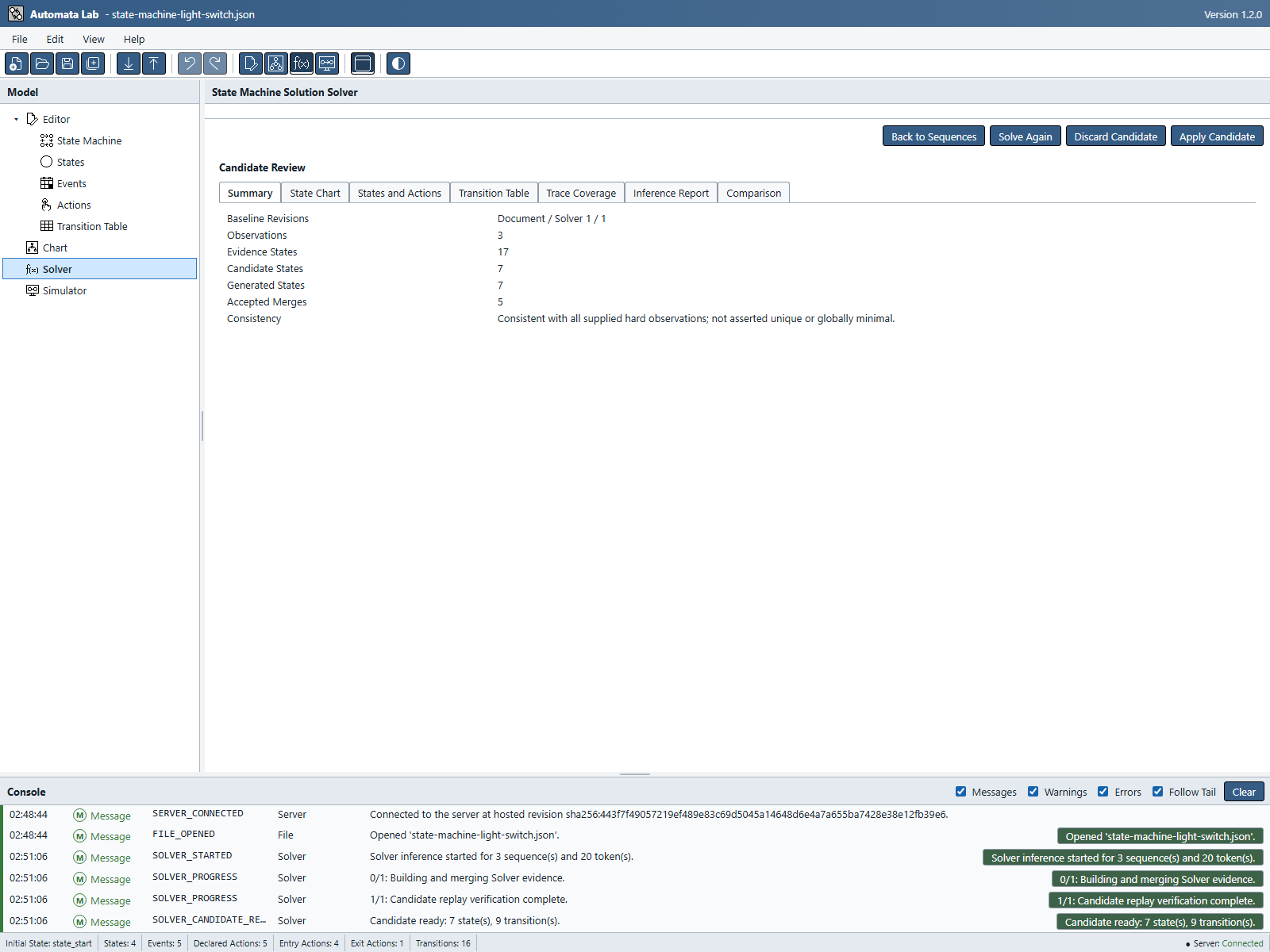
A successful Solve changes the page to Candidate Review without changing the project. Review these views:
| View | What to inspect |
|---|---|
| Summary | Baseline revisions, evidence and model counts, warnings, and the consistency statement. |
| State Chart | Read-only candidate structure with pan and zoom. |
| States and Actions | Complete ordered entry-action words and empty exit mappings. |
| Transition Table | Candidate transitions and observed or inferred provenance. |
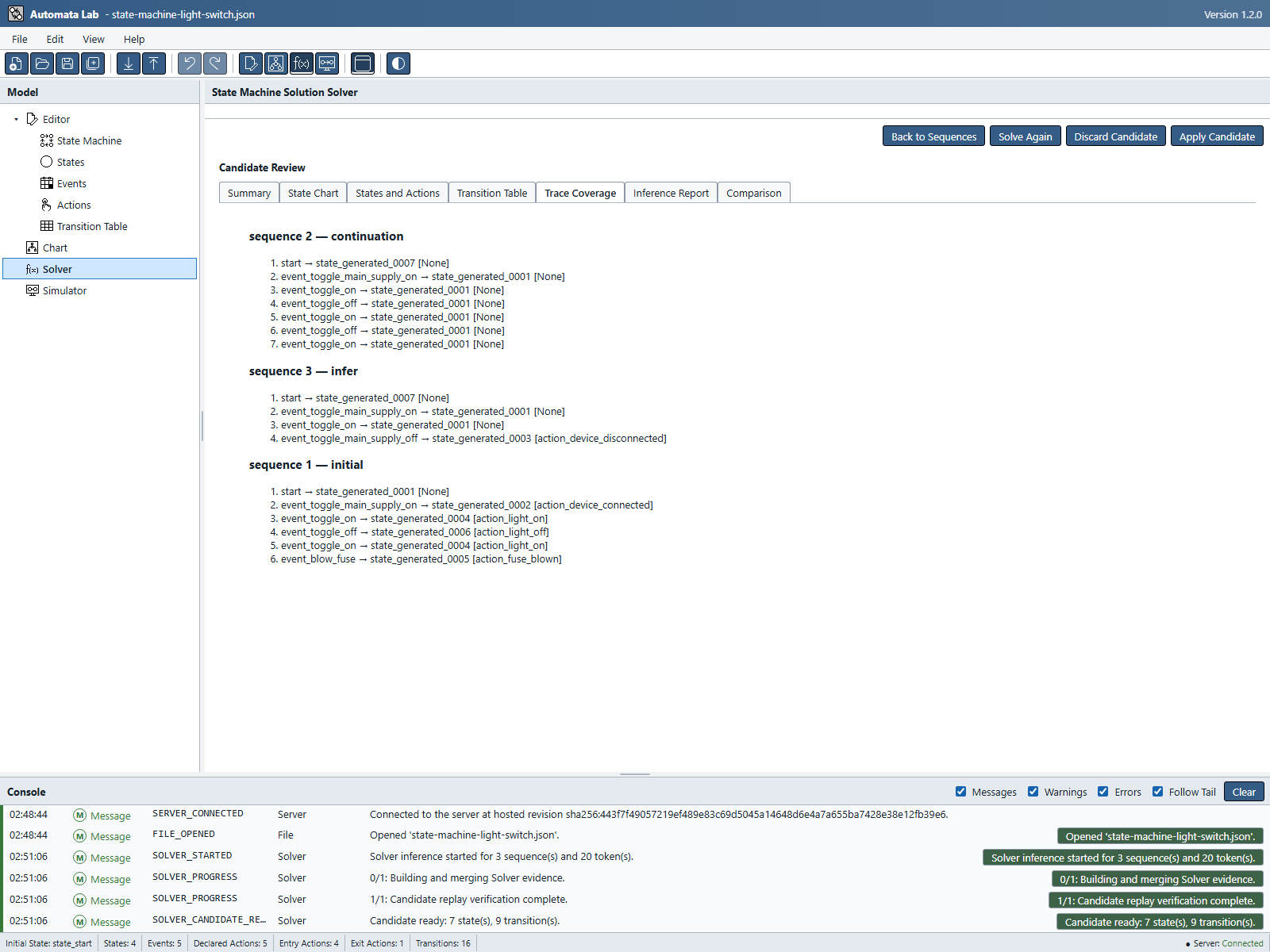
| Trace Coverage | Replay of every sample with interval-level matches. |
| Inference Report | Merges, generated states, weak starts, ambiguities, warnings, and tie-breaks. |
| Comparison | Current project versus candidate replacement impact. |
Choose the first view for future candidates in Application Settings → Solver → Results using Default Results Tab. The default is Summary. You can switch review tabs freely; changing the default does not move an existing candidate to another tab.
Figure UG-16 shows the result of solving the example's three observations. These counts describe this evidence set, not a minimum-state guarantee.
The candidate Chart uses top-to-bottom layered flow, with the initial state first and newly reached states below it. Mouse-wheel zoom centers on the pointer; left-button drag pans. Plus, Minus, arrow keys, and Home provide keyboard zoom, pan, and reset. Expand Chart States and the wrapping preferences change only the view and do not stale the candidate.
Inference Reports and Replay Coverage
Trace Coverage is the acceptance evidence for the candidate: every hard sample must replay successfully before Apply is offered. Inspect each interval's event, optional state identity, and complete ordered action word.
The Inference Report explains what was not directly observed. It includes generated identities, accepted and rejected merges, inferred initial decisions, weakly evidenced or unreachable fragments, ambiguity, and deterministic tie-breaks. Treat these disclosures as review points, especially when samples omit state names or begin with Infer or Continuation context.
In Figure UG-17, read sequence 1's ordered replay alongside its original tokens in Figure UG-14.
Applying or Discarding a Candidate
Use Back to Sequences to inspect the input while retaining the candidate, Solve Again to produce a replacement from current input, or Discard Candidate to remove the review result without changing the project.
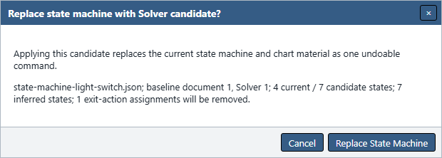
Apply Candidate opens a destructive replacement dialog. It names the project and baseline revisions, compares current and candidate counts, reports inferred states, and warns that the existing state machine, Chart, and exit-action assignments will be replaced. Confirm with Replace State Machine only after reviewing that impact.
Solver candidates set every terminal flag false: observations and the Simulator preference do not infer terminal membership. Summary, Comparison and Apply confirmation disclose the current terminal markings that will be removed. Undo restores the previous flags and exact indicator geometry. Figure UG-18 predates this additional terminal-marking disclosure; its other replacement fields remain applicable.
Apply is one local atomic undoable command. It replaces the semantic state machine and rebuilds Chart placement while preserving project metadata, Solver samples, and Simulator sequences. It does not Save the JSON project and does not Push anything to the hosted server.
Figure UG-18 shows the confirmation for this example. Review the loss of the existing exit assignment as well as the changed state count.
Stale Candidates
The candidate is bound to the project and Solver-input revisions used to produce it. Navigating away preserves a current candidate. Editing a sample marks it stale, and a changed project baseline prevents application.
A stale candidate remains useful for review but cannot replace the project. Choose Solve Again to produce a current candidate or Discard Candidate to remove it. This guard prevents an older inference result from overwriting newer authoring work.
CSV Import and Export
Use File → Import from CSV → Solver Observation Sequence to import one named sample. The CSV requires name and type columns. Each type must be event, state, or action; Automata Lab adds the matching canonical prefix when it is absent and rejects a conflicting prefix.
Import first asks for the destination sequence name. A collision produces one aggregate overwrite confirmation. The complete file is decoded, parsed, and validated before mutation; confirming a valid import applies it as one undoable command, while cancellation or any invalid row changes nothing.
Use File → Export to CSV → Solver Observation Sequence to write the selected sequence in current token order. Export uses canonical columns and CSV escaping. It does not change project revision, dirty state, JSON file association, or Undo history.
Previous: State Chart
Next: Server and Revisions